Basic Scripting Tutorial
In this first scripting tutorial, we will treat a simple use case of the theia library to design an optical bench. This tutorial may be a basis for developing more complex scripts, and aims at exposing the capabilities of the library.
To learn more on the classes and functions used here, please report to the (extensive) API documentation at the Documentation page.
Situation
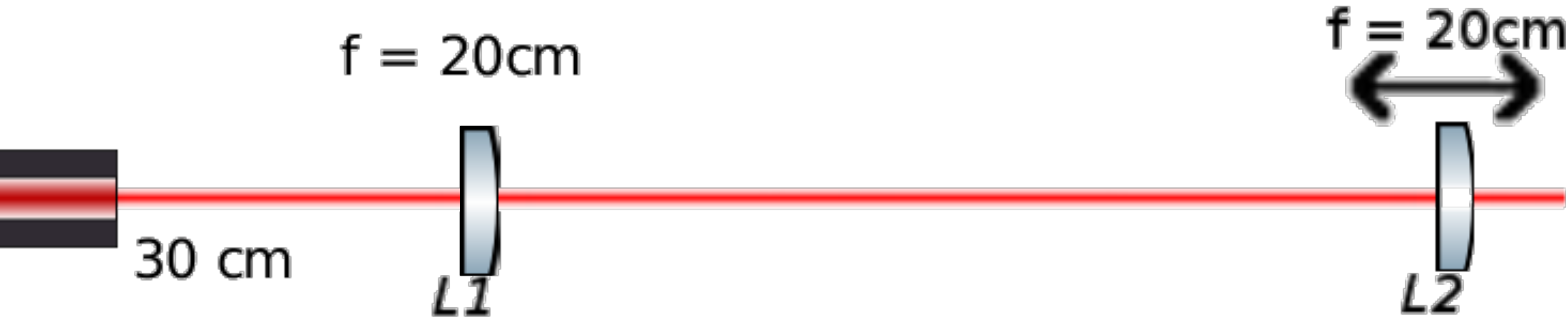
Imagine one has two converging lenses of (say) 20 cm of focal length and a laser placed (say) 30 cm in front of the first of these two lenses, as illustrated in the following figure. The laser and the first lens L1 are fixed in position by some other constraints of the optical bench, and L2 may be moved.
The question is:
What is the optimal position for lens L2, given that I want the beam output from the L1-L2 system to have the largest waist?
Or more generally:
Given a beam waist, may we find a position for lens L2 such that the beam output from the L1-L2 system has that given waist?
Algorithm
In order to solve this problem, we will use the theia library to implement the following algorithm:
Create a simulation object

Create sets to hold the results

Load this simulation with a laser object and a thin lens 20 cm focal lens

Choose a set of possible positions for L2

For every position in this set of positions:

     Create a 20 cm focal lens at this position

     Load this lens in the simulation

     Run the simulation

     Extract the waist of the beam transmitted by L2 and save it in the results

Plot the results
1. Importing the right tools
First, we must import the tools we will use for plotting (in our case we will use matplotlib). If we also want to write a CAD file at some time, we will need the FreeCAD libraries. Finally we import all packages of theia which are relevant to our case: simulation class, beams and thin lenses, units and settings. The Simulation class and settings are almost always mandatory because all simulations use a Simulation object and settings are used to initialize the global variables which can be used by the simulation functions.
#plotting stuff
import numpy as np
import matplotlib.pyplot as plt

#FreeCAD stuff
import sys
sys.path.append('/usr/lib/freecad/lib') # put the relevant path here
import FreeCAD as App
import Part

#theia stuff
from theia.helpers import settings
from theia.helpers.units import *
from theia.running import simulation
from theia.optics import thinlens, beam
2. Mandatory step: initialize the global variables
This step is always necessary because some functions of the simulation (such as the calculation of the daughter beams Gaussian parameters) use global variables in the command line tool. You can initialize them in the following way:
# initialize globals (necessary to use theia in library form)
dic = {'info': True, 'warning': True, 'text': True, 'cad': True,
		'fname': 'optimization', 'fclib' : '/usr/lib/freecad/lib',
        'antiClip': True, 'short': False}
settings.init(dic)
You can use this dictionary which works in any case. The fname variable is the name of the output files (if you choose to write any).
3. Creating the simulation object, the first lens and the beam
We use the constructor of the Simulation class and specify the order (an 0 order simulation is enough for us because we only want transmitted beams) and the threshold of the simulation. The names of the simulation (LName and FName) are not important here.
#simulation object
simu = simulation.Simulation(FName = 'optimization')
simu.LName = 'Optimizing with theia!'
simu.Order = 0
simu.Threshold = 0.5*mW
Then, we use the constructor of the ThinLens class and the user constructor of Gaussian beams to obtain L1 and the input beam.
#optics, the first L1 lens doesn't move
L1 = thinlens.ThinLens(X = 0*cm, Y = 0., Z = 0., Focal = 20.*cm,
			Diameter = 3.*cm, Phi = 180.*deg, Ref = 'L1')

bm = beam.userGaussianBeam(1.*mm, 1.*mm, 0., 0, 1064*nm, 1*W,
							X = -30*cm, Phi = 0, Ref = 'Beam')
Remember that all constructors have complete default values, which can be found in the Quick Reference guide. Here for example the X = 0*cm was not necessary. Notice the use of units provided by the units module we imported earlier.
4. Determine the optimization set
Now we provide the sets of all positions for L2 we want to optimize on. We also create two lists waistSizes and waistPositions to hold the results of the simulations.
# this is a list of centers for the second lens we want to try (it is around
#70 cm = L1.X + 2*Focal to respect the 2F configuration). We're trying n
#configurations around L2.X = 50
n = 50
centers = [ 40.*cm + 2.*cm*(float(i)/n) for i in range(-n, n)]
waistSizes = []
waistPositions = []
In this case, the optimization set is made of 100 positions around 40 cm (which is the 2F configuration position).
5. Perform the iterative optimization and extract the data
a. Load the input beam
First, we load the beam in the input beams of the simulation object once and for all.
# load beam
simu.InBeams = [bm]
b. Iterate the simulation over all possibilities for L2
Then, we iterate over all the possible positions (centers) of the L2 lens by creating a thin lens of focal 20 cm at the position and loading this lens and L1 into the optics list (OptList) of the simulation object.
For each of the positions, we run the simulation.
#run the simulations in sequence!
for center in centers:
	dic = {'X': center, 'Y': 0., 'Z': 0., 'Focal': 20.*cm,
		'Diameter': 3.*cm, 'Theta': 90*deg, 'Phi': 180.*deg, 'Ref': 'L2'}
	simu.OptList = [L1, thinlens.ThinLens(**dic)]

	#go theia go!
	simu.run()
Now that the simulation has occurred and the new beams have populated the simulation’s beam trees, we can extract the Gaussian data of the output beam and save it in our lists of waist widths and positions for plotting later.
c. Make a reference to the output beam for treatment
The output beam is the beam transmitted by the L1-L2 system of the first input beam of the simulation. Thus, it is the Root object (beam) of the T.T.T.T beam tree (transmitted by the two surfaces of L1 and the two surfaces of L2, thus 4 times transmitted) of the first member of the simulation beam tree list.
output = simu.BeamTreeList[0].T.T.T.T.Root #beam of the 4-transmitted daughter tree of the first input beam
d. Calculate the Gaussian parameters and save them
Now that we have a reference to the beam, we use the Gaussian functions waistSize and waistPos of the beam (and keep only the values on X, hence the [0]) to store the relevant data in our lists of results.
	#save output data for plotting
	waistSizes.append(output.waistSize()[0])
	waistPositions.append(output.waistPos()[0])
6. Plotting the results
Now that we have iteratively populated the results sets with the widths (and positions) of the waist of the output beams, we can plot the results however we like.
First, let us write the CAD file. This file will of course only contain the information of the last iteration results, because each new run re-initializes the beam trees (but not the input beams). The writeCAD method of the simulation object is called to write the CAD file.
simu.writeCAD()
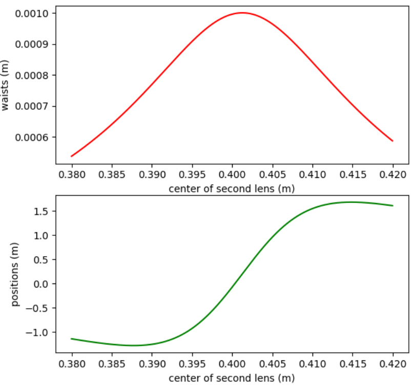
Next, we plot the results of widths and positions as a function of the position of L2 with matplotlib. We can then read the optimal position of L2 to solve our problem.
#plot the results
plt.figure(1)
plt.subplot(211)
plt.plot(centers, waistSizes, 'r')
plt.ylabel('waists (m)')
plt.xlabel('center of second lens (m)')
plt.subplot(212)
plt.plot(centers, waistPositions, 'g')
plt.ylabel('positions (m)')
plt.xlabel('center of second lens (m)')
plt.show()
In the case of a 1 mm input beam, the results are given by the following graphs. It is easy to notice that the 2F configuration is optimal for the width.
Troubleshooting
You may run into some errors while scripting with theia. The most common errors encountered are:
KeyError: [some key of the init method]: You have not initialized all the global variables (use the snippet from step 2 of this tutorial, it always works).AttributeError: 'NoneType' object has no attribute 'T' [or 'R']: One tree has no daughter (NoneType) and you are accessing the daughter tree (TorR) of that non-existing tree. Make sure you have correctly input the optics and that all the beams you expected were traced. You can find out how many beams where traced using thenumberOfBeamsmethod of the BeamTree class. For example:
simu.BeamTreeList[0].numberOfBeams() #number of beams of the first beam tree of the simulation object